J-SpaceStudy Notes

Over the past few days, I have been studying Anthropic's work, published this July, on visualizing a model's global workspace. I found it very inspiring, so I wanted to write down my understanding and thoughts.

Abstract

This note uses a theater analogy to introduce the global workspace, leading into the central idea of Anthropic's article: how can we observe a large language model's "global workspace"? We will first look at how their tools for observing and intervening on intermediate representations, J-Lens and J-Space, work. Then we will see how the researchers use these tools and their experiments to argue that large language models may have a global workspace, and to explore some of its interesting properties. Finally, I will share some of my own thoughts and questions about the article.

Global Workspace Theory

In 1988, one of the clouds hanging over cognitive science was this question: why can we consciously report some of our brain's activity, while remaining unaware of other activity? The invisible gorilla experiment (Simons, 1999) illustrates this very well. If you are unfamiliar with it, take a look at this video:

Watch the gorilla experiment ↗

In the gorilla experiment, the visual input clearly includes the pixels of the gorilla, and these pixels are processed by the visual cortex. Yet they are not captured by awareness. The experiment gives us a simple demonstration that not every signal enters consciousness. So how does the brain process information? This was one of the puzzles facing cognitive science.

To address this question, Bernard Baars proposed one possible explanation: Global Workspace Theory (GWT, Baars, 1988).

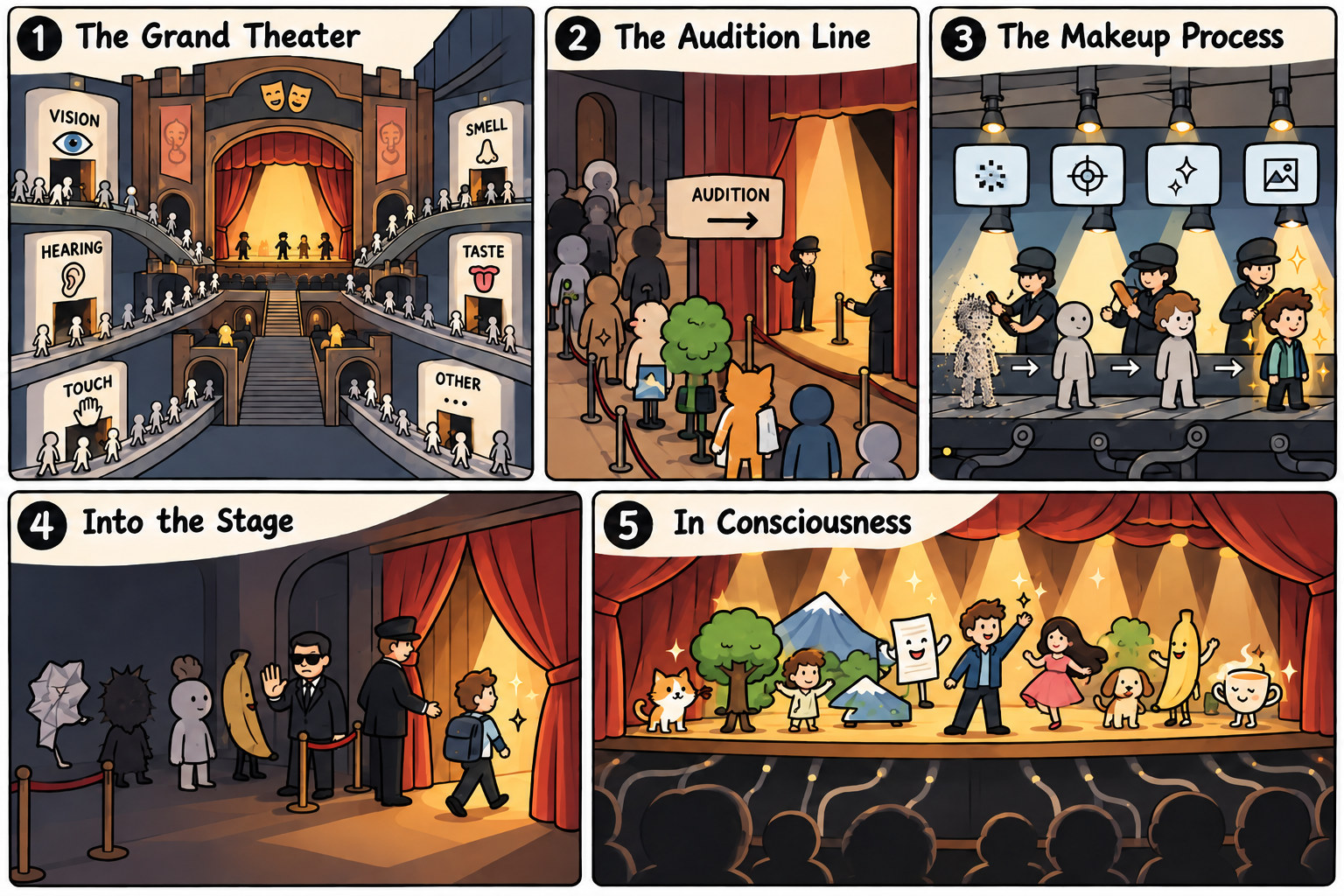
The theory gives us a vivid picture. The whole cognitive system is like a large theater, and the central stage is the global workspace. The props and actors on this stage are the things we can consciously perceive. Of course, this is a very unusual theater: it is a cognitive system, after all! The audience surrounding the stage corresponds to the brain circuits that specialize in different kinds of information processing.

Our brains constantly process information from the body: the smell of a pleasant fragrance, the touch of keys under our fingers, the sight of a leaf's texture, the sound of someone shouting by the road, or the subtle taste of tea. Various small circuits or functions process this information, which competes for a place on the stage.

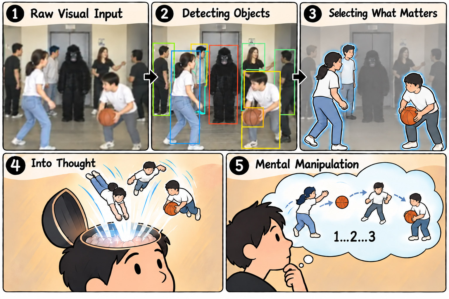
Imagine these circuits as skilled makeup artists preparing aspiring actors who run along the central avenue into the theater. Returning to the invisible gorilla experiment, some applicants never even get through the door, such as things outside the screen. Some look like natural stars, such as the players in white. There are also many supporting performers, such as the players in black, and others who enter the theater but never make it onto the stage, such as the gorilla.

The makeup artists, our small brain processors, prepare the actors one by one. The applicants move through successive stages of this production line. By the time they reach the stage, they have gone from an unadorned appearance to smart suits and full makeup. If the stage selector thinks an actor stands out, they are allowed onstage. Those who are too inconspicuous may be turned away.

The corresponding process might be visual information starting as a noisy input, becoming clearer through processing, and having its most eye-catching elements sent onto the stage first, entering awareness. Once onstage, these actors become objects that consciousness can observe and manipulate, through reasoning, translation, or rotation.

What makes this a global workspace is broadcasting: once information enters the stage, multiple specialized processing systems around it can read and use it together. These systems handle not only external sensory input, but also memory, reasoning, decision-making, and language.

For example, seeing dark clouds over a mountain might remind the memory system of getting caught in the rain, prompt the decision-making system to consider heading downhill, and let the language system form the sentence, "It might rain." Reaching the stage therefore means both entering awareness and becoming available for flexible use by multiple systems.

That is the global workspace: a stage for the concepts we can observe and manipulate in our conscious experience.

A Global Workspace in Large Language Models? J-Lens and J-Space

The central idea of the J-Space article is that large language models may have something resembling a global workspace, or GW. How could we establish that such a workspace exists in a model? It would lie somewhere in the successive Transformer blocks, but how could we argue that these hard-to-interpret intermediate layers constitute a GW?

The article introduces two concepts: J-Lens and J-Space.

J-Lens lets us examine the state of a model's GW at a particular moment. J-Space gives a mathematical definition of a state space formed by the representations this method can read. We can think of it as an approximate, readable state space of the GW. I will introduce them one by one.

J-Lens: a Magnifying Glass for the Actors on Stage

If we want to know whether a layer has workspace-like properties, we need a way to identify its actors. J-Lens is our tool for looking at them.

J-Lens is defined as follows:

Here, $h_{\ell, t}$ is the hidden state at layer $\ell$ and sequence position $t$ of the Transformer block.

The formula may look intimidating, but its meaning is simple: what influence does the Transformer block at layer $\ell$ have on the future, on average?

Step 1 Compute position-to-position influence Step 2 Aggregate across positions and prompts

First, see how a change at one position affects the current and later positions.

Next step →

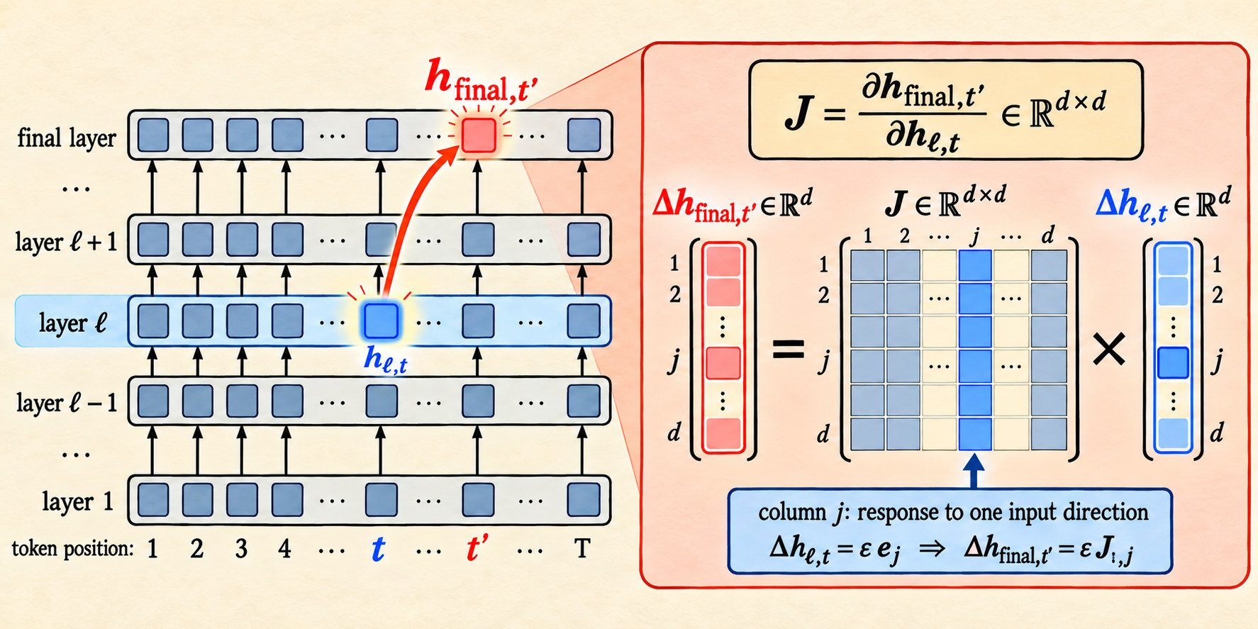
First, look inside the formula. $\frac{\partial h_{\text {final }, t^{\prime}}}{\partial h_{\ell, t}}$ describes how a small change to the hidden state at layer $\ell$, position $t$, affects the final-layer hidden state at position $t'$. This is what the arrows in the Step 1 image represent: they connect one intermediate-layer position to different positions in the final layer.

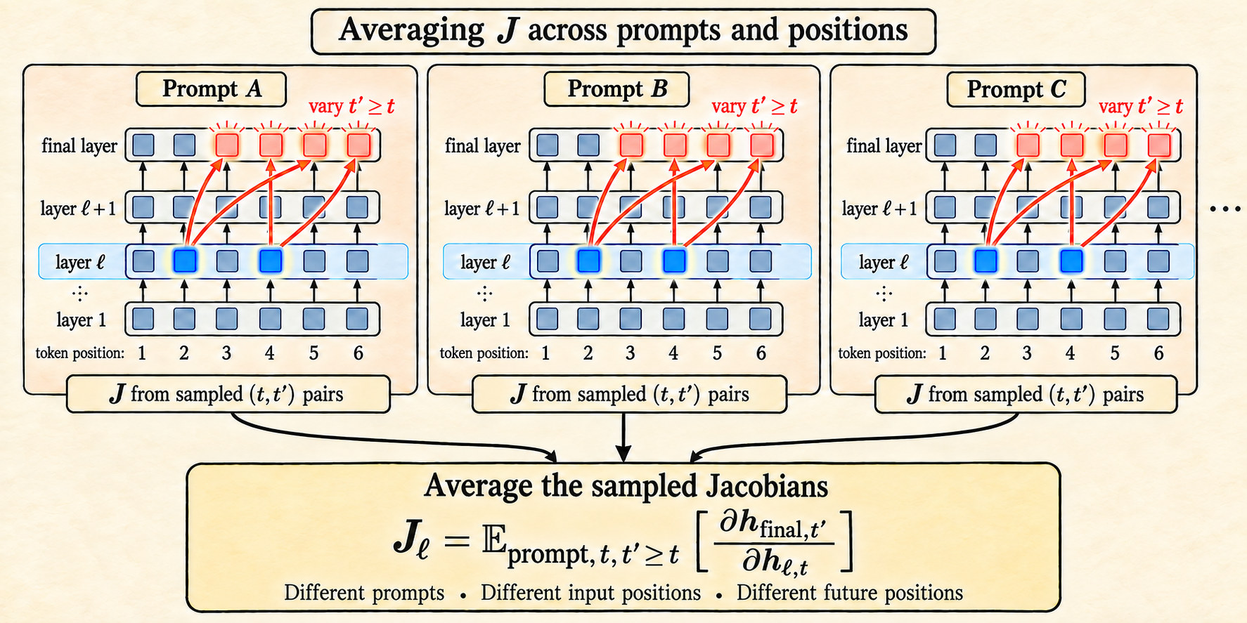
Now look at the outer $\mathbb{E}_{t,\,t^{\prime}\geq t,\,\text{prompt}}$ term. The expectation notation summarizes the aggregation of influences across different $t$, $t'$, and prompts. In the actual calculation, we first sum a given position's influences on the current and subsequent positions, then average over source positions, and finally over prompts, obtaining $J_\ell$. This corresponds to the Step 2 image, where Jacobians calculated for different positions and prompts are brought together.

So, taken together, it captures the average influence of layer $\ell$ on the future.

In practice, the researchers compute Jacobians for different source and target positions within a variety of prompts. Expanding the formula according to the actual aggregation procedure: first sum all influences from a given position $t$ to the current and subsequent positions, then average over source positions $t$, and finally average over prompts.

Using J-Lens

Readout

Of course, obtaining the matrix $J_\ell$ alone does not directly give us a readable output.

Take a hidden state at any layer and position, transform it with $J_\ell$, apply RMS normalization, multiply by the unembedding matrix, and finally apply softmax. This gives us a distribution over words. In a formula:

The highest-ranked words help us identify prominent concepts in the current hidden state that can be expressed in language. They reveal information about the actors at this layer and moment $t$; we can naturally treat the text sequence as a kind of time. In this way, J-Lens can inspect the actors at any layer and moment.

There is one caveat here. This word distribution cannot directly be treated as the probability that the model believes a particular claim; rather, we can intuitively think of it as how likely a word is to represent a concept, or actor, being considered in this layer's workspace. That wording is not entirely precise, but it offers an intuitive way to think about it. For instance, reading out spider tells us that a spider-related concept is present. The model might be considering spider as the answer, ruling it out, or comparing spiders with ants. The word alone does not distinguish these possibilities. To understand what the actor is doing, we need the context and the intervention experiments that follow.

In the paper's experiments with Claude Sonnet 4.5, J-Lens finds mostly sensory information from $L_{0}$ to $L_{38}$, with very noisy readouts. From $L_{38}$ to $L_{92}$, essentially every layer acts as a workspace, while from $L_{92}$ to $L_{100}$, the readout becomes increasingly similar to the output. Here, $L$ is a percentage of model depth; it does not mean Claude literally has 100 layers.

Sparse Decomposition

Besides directly inspecting the readout, we can use sparse decomposition: approximately expressing the current hidden state as a nonnegative weighted sum of a small number of J-Lens vectors. This reads and decomposes an existing activation; it does not change the model's state.

The procedure is also straightforward:

Here, $v_i$ is the J-Lens vector corresponding to row $i$ of the matrix $W_U J_\ell$. Using the convention that hidden states are column vectors, if $u_i$ is the transpose of row $i$ of the unembedding matrix $W_U$, then $v_i = J_\ell^\top u_i$.

In other words, we pull an output token's readout direction back into the hidden-state space of layer $\ell$, rather than mapping it forward with $J_\ell$. We then choose at most $k$ vectors $v_i$ and find nonnegative weights that approximate $h$ in Euclidean distance.

We first obtain directions corresponding to vocabulary tokens, then jointly choose directions and weights to minimize reconstruction error. This is not simply selecting the $k$ highest-scoring readout words, because the directions are not orthogonal. After decomposition, $\lVert \alpha_i v_i \rVert$ describes the size of each contribution.

But sparse decomposition has a larger use beyond readout: perturbing the model's state, or inception.

Inception

J-Lens is more than a magnifying glass. Its vectors can also change a hidden state at a particular layer. I call this writing intervention Inception, after the film.

Writing

There are two methods. The first directly selects the J-Lens vector for a target token, multiplies it by a strength coefficient, and adds it to $h$. This does not require sparse decomposition first.

The second selects the J-Lens vectors for a source token $s$ and target token $t$, placing them in the two columns of $V=[v_s\;v_t]$. A pseudoinverse gives the coordinates of $h$ in the space spanned by these vectors: $c=V^{\dagger}h$, where $V^{\dagger}$ is the pseudoinverse of $V$.

Next, swap the two coordinates in $c$. Subtract the original component of $h$ in this space and add back the component with swapped coordinates. In a formula:

Here, $\sigma$ swaps the two coordinates. To adjust intervention strength, we can also multiply the difference $\sigma(c)-c$ by a coefficient $\alpha$. The part of $h$ perpendicular to $\operatorname{span}\{v_s,v_t\}$ remains unchanged. Neither vector has to appear in the sparse decomposition of $h$.

Notice that this does not exactly coincide with readout.

In the actual injection or swap, the operation is applied at every position in the layer.

J-Space

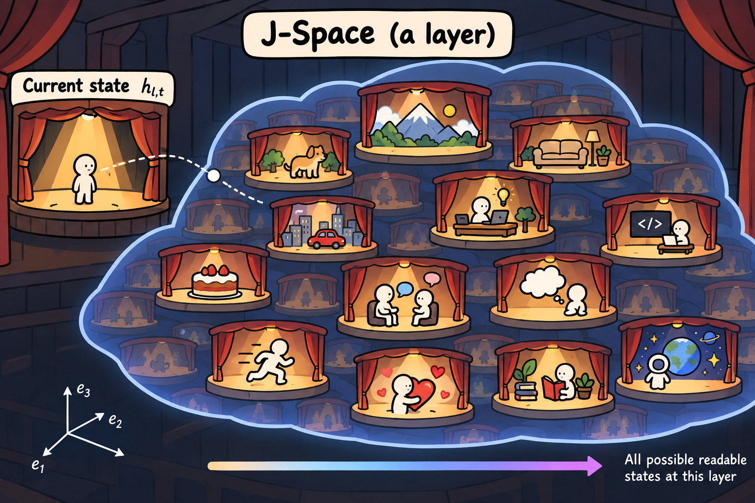
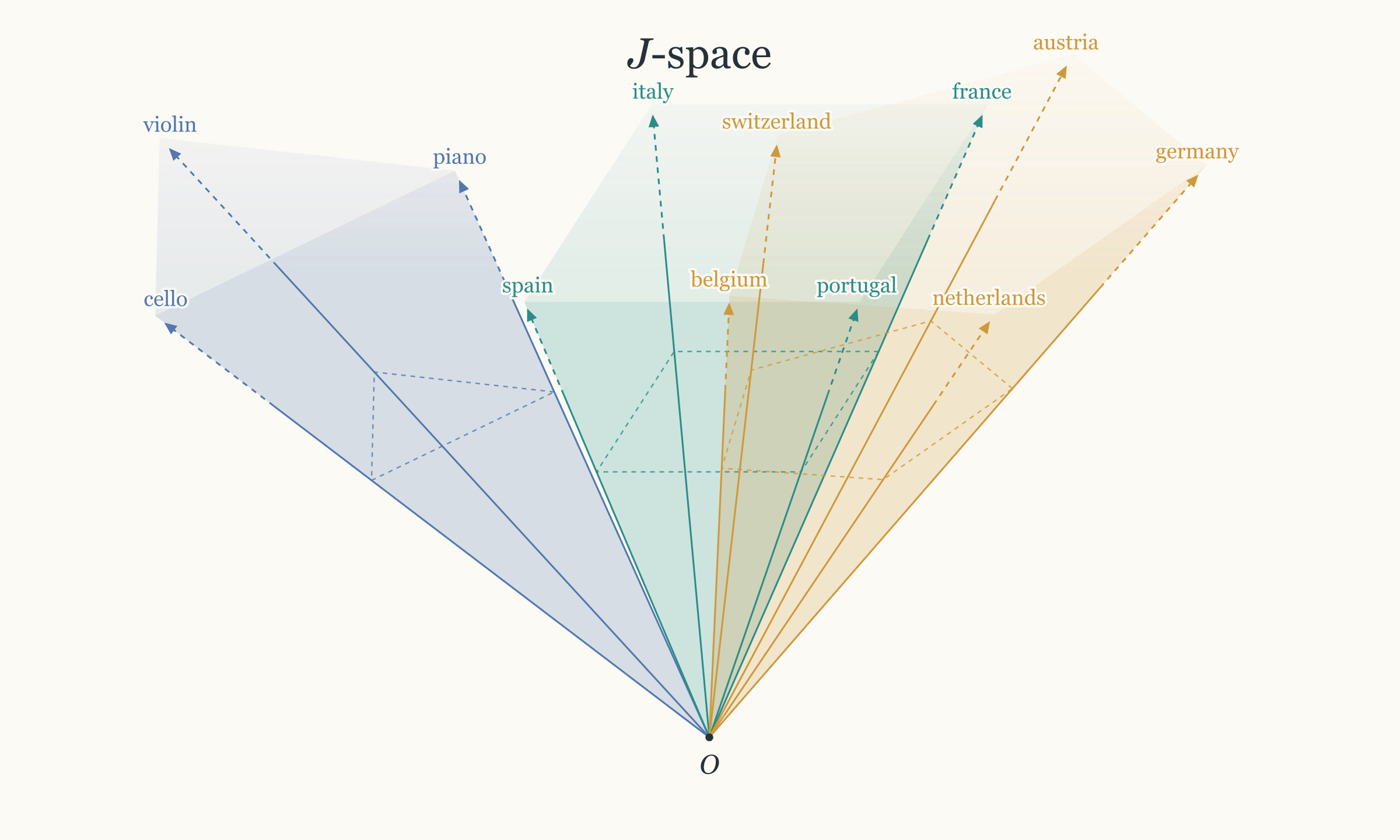
J-Space is essentially the search space for sparse decomposition, given a set of J-Lens vectors and sparsity $k$. When doing sparse decomposition, we look for a point in J-Space that is as close as possible to $h$ in Euclidean distance. Each point is a nonnegative combination of at most $k$ word directions, corresponding to a candidate combination of actors.

In other words, J-Space is an approximate, readable state space for the stage at a given layer. These candidate combinations of actors are not guaranteed to cover everything in the model's workspace, and not every combination is necessarily a state the model will actually reach.

We might imagine the shape of this set as follows:

Experiments

We have now introduced the article's basic tools and principles. What remains is to see which experiments support the possibility that the model really has a global workspace.

I think four experiments are especially worth introducing.

The first experiment tests whether these layers really have workspace-like functions.

The model's prompt says, "I can inject a thought into your mind. What do you think it is?" It is then required to begin its answer with: "I do detect it. The thought is:"

At layer 88, the readout is elephant, and the final prediction is also elephant. When the writing method injects lightning into the model, its next-token prediction changes to lightning.

I would have liked the article to show more of what other layers are thinking about here, to help us understand what is happening elsewhere in the model.

The researchers also ask the model to write about one thing while thinking about something else.

The second experiment shows that J-Space participates in reasoning. In one example, the model is asked how many legs a web-spinning animal has. Spider appears in J-Space, and the model initially answers 8.

Using the swapping method described earlier, the researchers exchange the activation's coordinates along the spider and ant J-Lens directions in an intermediate layer. The model then answers 6. We are therefore doing more than observing the word spider: changing this intermediate representation also changes the final answer, indicating a causal role in the reasoning result.

The third experiment demonstrates generalization of concepts in J-Space. In separate questions about France's capital, language, and continent, the researchers swap the coordinates along the France and China J-Lens vectors in an intermediate layer. They use exactly the same swap for the different questions.

In this example, the answers shift to China's capital, language, and continent. The key is that the same substituted concept can be used by different downstream computations, rather than merely reading out different words for different questions. In larger-scale tests, these swaps do not succeed every time.

The fourth experiment examines selectivity in J-Space. We have seen that changing the actors on stage can change an answer. Now we ask whether every use of the same information must pass through this stage. The researchers give the model a Spanish passage, then swap the coordinates along the Spanish and French J-Lens directions at the question's token positions.

Asked which language the passage is in, the model changes its answer from Spanish to French. Asked to name a famous author who writes in that language, it also shifts to a French author.

But asked to continue the passage, it still writes Spanish. If a French sentence is inserted into the passage and the model is asked to check for a language switch, it can still detect the anomaly.

Across these tasks, the actor in J-Space affects answers when the model reports the language or uses it to name an author. Continuing the text and detecting an inserted language still work normally after the same swap.

This suggests that even when the same concept appears in the readout, different tasks do not necessarily use its J-Space representation. That is the selectivity at issue here, and it helps reveal a functional difference between the stage and other processing. Interested readers can see Figure 20 in the original article.

The article contains many other interesting experiments: showing that J-Space vectors are more sensitive to writing interventions, observing the model thinking about one thing while writing another, and watching reasoning evolve in the workspace during calculations. I highly recommend reading the original.

This note is mainly a reading guide.

Questions and Criticisms

My main questions about this method concern J-Space.

First, we should distinguish two possible forms of non-uniqueness. The J-Lens vectors form an overcomplete dictionary, so the same vector may admit several coefficient sets. Meanwhile, J-Space under a sparsity constraint is generally nonconvex, so a given hidden state may also have more than one nearest point. These are different issues, and nonconvexity alone does not imply that every hidden state has multiple optimal decompositions. What concerns me more is whether the sparse decomposition of the same hidden state is stable.

Second, sparse decomposition requires us to choose not only a set of word directions but also nonnegative weights $\alpha$. Mathematically, $\alpha$ is simply a reconstruction weight. What gives me pause is that we can change both the words and their weights, opening up more possible choices.

When some word directions are already close together, a different combination of words and weights might approximate the hidden state almost equally well.

So I care about how stable the final set of words is. If we use a different solver or perturb the hidden state slightly, do we get another set of words, with large changes even in the contribution sizes represented by $\lVert \alpha_i v_i \rVert$?

Of course, more choices do not necessarily mean multiple solutions. But a small reconstruction error alone does not answer these stability questions.

Simons, D. J., & Chabris, C. F. (1999). Gorillas in our midst: Sustained inattentional blindness for dynamic events. Perception, 28(9), 1059–1074.